第三章 线性神经网络

def synthetic_data(w, b, num_examples):
    """生成 y = Xw + b + 噪声"""
    X = torch.normal(0, 1, (num_examples, len(w)))
    y = torch.matmul(X, w) + b
    y += torch.normal(0, 0.01, y.shape)
    return X, y.reshape((-1, 1))

true_w = torch.tensor([2, -3.4])
true_b = 4.2
features, labels = synthetic_data(true_w, true_b, 1000)

def data_iter(batch_size, features, labels):
    num_examples = len(features)
    indices = list(range(num_examples))
    # 样本随机读取，没有特定的顺序
    random.shuffle(indices)
    for i in range(0, num_examples, batch_size):
        batch_indices = torch.tensor(
            indices[i: min(i + batch_size, num_examples)])
        yield features[batch_indices], labels[batch_indices]

w = torch.normal(0, 0.01, size=(2,1), requires_grad=True)
b = torch.zeros(1, requires_grad=True)

def linreg(X, w, b):
    """线性回归模型"""
    return torch.matmul(X, w) + b

def squared_loss(y_hat, y):
    """均方损失"""
    return (y_hat - y.reshape(y_hat.shape)) ** 2 / 2

def sgd(params, lr, batch_size):
    """小批量随机梯度下降"""
    with torch.no_grad():
        for param in params:
            param -= lr * param.grad / batch_size
            param.grad.zero_()

lr = 0.03
num_epochs = 3
net = linreg
loss = squared_loss

for epoch in range(num_epochs):
    for X, y in data_iter(batch_size, features, labels):
        l = loss(net(X, w, b), y)  # X 和 y 的小批量损失
        # 因为 l 形状是 (batch_size,1)，而不是一个标量。l 中的所有元素被加到一起，
        # 并以此计算关于 [w, b] 的梯度
        l.sum().backward()
        sgd([w, b], lr, batch_size)  # 使用参数的梯度更新参数
    with torch.no_grad():
        train_l = loss(net(features, w, b), labels)
        print(f'epoch {epoch + 1}, loss {float(train_l.mean()):f}')

import numpy as np
import torch
from torch.utils import data
from d2l import torch as d2l

true_w = torch.tensor([2, -3.4])
true_b = 4.2
features, labels = d2l.synthetic_data(true_w, true_b, 1000)

def load_array(data_arrays, batch_size, is_train=True):
    """构造一个 PyTorch 数据迭代器"""
    dataset = data.TensorDataset(*data_arrays)
    return data.DataLoader(dataset, batch_size, shuffle=is_train)

batch_size = 10
data_iter = load_array((features, labels), batch_size)

# nn 是神经网络的缩写
from torch import nn

net = nn.Sequential(nn.Linear(2, 1))

net[0].weight.data.normal_(0, 0.01)
net[0].bias.data.fill_(0)

loss = nn.MSELoss()

trainer = torch.optim.SGD(net.parameters(), lr=0.03)

num_epochs = 3
for epoch in range(num_epochs):
    for X, y in data_iter:
        l = loss(net(X) ,y)
        trainer.zero_grad()
        l.backward()
        trainer.step()
    l = loss(net(features), labels)线性模型
    print(f'epoch {epoch + 1}, loss {l:f}')

%matplotlib inline
import torch
import torchvision
from torch.utils import data
from torchvision import transforms
from d2l import torch as d2l

d2l.use_svg_display()

# 通过 ToTensor 实例将图像数据从 PIL 类型变换成 32 位浮点数格式，
# 并除以 255 使得所有像素的数值均在 0～1 之间
trans = transforms.ToTensor()
mnist_train = torchvision.datasets.FashionMNIST(
    root="../data", train=True, transform=trans, download=True)
mnist_test = torchvision.datasets.FashionMNIST(
    root="../data", train=False, transform=trans, download=True)

def get_fashion_mnist_labels(labels):
    """返回 Fashion-MNIST 数据集的文本标签"""
    text_labels = ['t-shirt', 'trouser', 'pullover', 'dress', 'coat',
                   'sandal', 'shirt', 'sneaker', 'bag', 'ankle boot']
    return [text_labels[int(i)] for i in labels]

def show_images(imgs, num_rows, num_cols, titles=None, scale=1.5):
    """绘制图像列表"""
    figsize = (num_cols * scale, num_rows * scale)
    _, axes = d2l.plt.subplots(num_rows, num_cols, figsize=figsize)
    axes = axes.flatten()
    for i, (ax, img) in enumerate(zip(axes, imgs)):
        if torch.is_tensor(img):
            # 图片张量
            ax.imshow(img.numpy())
        else:
            # PIL 图片
            ax.imshow(img)
        ax.axes.get_xaxis().set_visible(False)
        ax.axes.get_yaxis().set_visible(False)
        if titles:
            ax.set_title(titles[i])
    return axes

def get_dataloader_workers():
    """使用 4 个进程来读取数据"""
    return 4

def load_data_fashion_mnist(batch_size, resize=None):
    """下载 Fashion-MNIST 数据集，然后将其加载到内存中"""
    # 通过 ToTensor 实例将图像数据从 PIL 类型变换成 32 位浮点数格式
    trans = [transforms.ToTensor()]
    # 使用 resize 将图像调整到另一种形状
    if resize:
        trans.insert(0, transforms.Resize(resize))
    trans = transforms.Compose(trans)
    # 下载数据集
    mnist_train = torchvision.datasets.FashionMNIST(
        root="../data", train=True, transform=trans, download=True)
    mnist_test = torchvision.datasets.FashionMNIST(
        root="../data", train=False, transform=trans, download=True)
    # 返回内置数据迭代器
    return (data.DataLoader(mnist_train, batch_size, shuffle=True,
                            num_workers=get_dataloader_workers()),
            data.DataLoader(mnist_test, batch_size, shuffle=False,
                            num_workers=get_dataloader_workers()))

train_iter, test_iter = load_data_fashion_mnist(32, resize=64)
for X, y in train_iter:
    print(X.shape, X.dtype, y.shape, y.dtype)
    break

import torch
from IPython import display
from d2l import torch as d2l

batch_size = 256
train_iter, test_iter = d2l.load_data_fashion_mnist(batch_size)

num_inputs = 784    # 28*28 的图像视为一维向量
num_outputs = 10    # 对应 10 个类别

W = torch.normal(0, 0.01, size=(num_inputs, num_outputs), requires_grad=True)   # 784*10
b = torch.zeros(num_outputs, requires_grad=True)    # 1*10

def softmax(X):
    X_exp = torch.exp(X)
    partition = X_exp.sum(1, keepdim=True)
    return X_exp / partition

def net(X):
    return softmax(torch.matmul(X.reshape(-1, W.shape[0]), W) + b)

def cross_entropy(y_hat, y):
    return - torch.log(y_hat[range(len(y_hat)), y])

def accuracy(y_hat, y):
    """计算预测正确的数量"""
    if (len(y_hat.shape) > 1) and (y_hat.shape[1] > 1):
        y_hat = y_hat.argmax(axis=1)
    cmp = y_hat.type(y.dtype) == y
    return float(cmp.type(y.dtype).sum())

def evaluate_accuracy(net, data_iter):
    """计算在指定数据集上模型的精度"""
    if isinstance(net, torch.nn.Module):
        net.eval()  # 将模型设置为评估模式
    metric = d2l.Accumulator(2)  # 正确预测数、预测总数
    with torch.no_grad():
        for X, y in data_iter:
            metric.add(accuracy(net(X), y), y.numel())
    return metric[0] / metric[1]

def train_epoch_ch3(net, train_iter, loss, updater):
    """训练模型一个迭代周期（定义见第 3 章）"""
    # 将模型设置为训练模式
    if isinstance(net, torch.nn.Module):
        net.train()
    # 训练损失总和、训练准确度总和、样本数
    metric = Accumulator(3)
    for X, y in train_iter:
        # 计算梯度并更新参数
        y_hat = net(X)
        l = loss(y_hat, y)
        if isinstance(updater, torch.optim.Optimizer):
            # 使用 PyTorch 内置的优化器和损失函数
            updater.zero_grad()
            l.mean().backward()
            updater.step()
        else:
            # 使用定制的优化器和损失函数
            l.sum().backward()
            updater(X.shape[0])
        metric.add(float(l.sum()), accuracy(y_hat, y), y.numel())
    # 返回训练损失和训练精度
    return metric[0] / metric[2], metric[1] / metric[2]

def train_ch3(net, train_iter, test_iter, loss, num_epochs, updater):
    """训练模型（定义见第 3 章）"""
    animator = d2l.Animator(xlabel='epoch', xlim=[1, num_epochs], ylim=[0.3, 0.9],
                        legend=['train loss', 'train acc', 'test acc'])
    for epoch in range(num_epochs):
        train_metrics = train_epoch_ch3(net, train_iter, loss, updater)
        test_acc = evaluate_accuracy(net, test_iter)
        animator.add(epoch + 1, train_metrics + (test_acc,))
    train_loss, train_acc = train_metrics
    assert train_loss < 0.5, train_loss
    assert train_acc <= 1 and train_acc > 0.7, train_acc
    assert test_acc <= 1 and test_acc > 0.7, test_acc

lr = 0.1

def updater(batch_size):
    return d2l.sgd([W, b], lr, batch_size)

num_epochs = 10
train_ch3(net, train_iter, test_iter, cross_entropy, num_epochs, updater)

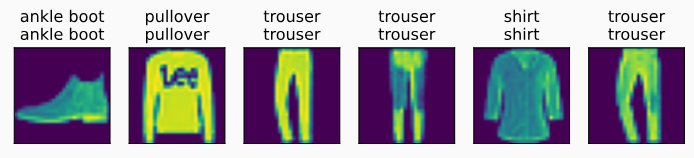
def predict_ch3(net, test_iter, n=6):
    """预测标签（定义见第 3 章）"""
    for X, y in test_iter:
        break
    trues = d2l.get_fashion_mnist_labels(y)
    preds = d2l.get_fashion_mnist_labels(net(X).argmax(axis=1))
    titles = [true +'\n' + pred for true, pred in zip(trues, preds)]
    d2l.show_images(
        X[0:n].reshape((n, 28, 28)), 1, n, titles=titles[0:n])

predict_ch3(net, test_iter)

import torch
from torch import nn
from d2l import torch as d2l

# 加载数据
batch_size = 256
train_iter, test_iter = d2l.load_data_fashion_mnist(batch_size)

# 定义网络
# PyTorch 不会隐式地调整输入的形状。因此，我们在线性层前定义了展平层（flatten），来调整网络输入的形状
net = nn.Sequential(nn.Flatten(), nn.Linear(784, 10))

def init_weights(m):
    if type(m) == nn.Linear:
        nn.init.normal_(m.weight, std=0.01)

net.apply(init_weights)

# 损失函数
# PyTorch 为交叉熵损失函数传递未规范化的预测，在函数中再计算 softmax 及其对数
loss = nn.CrossEntropyLoss(reduction='none')

# 优化器
trainer = torch.optim.SGD(net.parameters(), lr=0.1)

# 训练
num_epochs = 10
d2l.train_ch3(net, train_iter, test_iter, loss, num_epochs, trainer)