Linear Regression

0.1 General Expression

$$y_{i}=\beta_{0}+\beta_{1}\times x_{i1}+\cdots+\beta_{p}\times x_{ip}+\epsilon_{i},\quad i=1,2,\cdots,n$$ $$ \begin{align*} \mathbf{y}&=(y_{1},y_{2},\cdots,y_{n})^{T} \cr \mathbf{X}&=\begin{bmatrix}1 & x_{11} & x_{12} & \cdots & x_{1p} \cr 1 & x_{21} & x_{22} & \cdots & x_{2p} \cr \vdots & \vdots & \vdots & \vdots & \vdots \cr 1 & x_{n1} & x_{n2} & \cdots & x_{np} \end{bmatrix} \cr \mathbf{\beta}&=(\beta_{0},\beta_{1},\cdots,\beta_{p})^{T} \cr \mathbf{\epsilon}&=(\epsilon_{1}, \epsilon_{2},\cdots,\epsilon_{n})^{T} \end{align*} $$

0.2 OLS Assumptions

The regression model is parametric linear.
${x_{i1},x_{i2},\cdots,x_{ip}}$ are nonstochastic variables.
$E(\epsilon_{i})=0$.
$Var(\epsilon_{i})=\sigma^{2}$.
${\epsilon_{i}}$ are independent random variables, so as to say: no autocorrelation, $cov(\epsilon_{i},\epsilon_{j})=0,i\neq j$.
The regression model is set correctly, without setting bias.

0.3 OLS Estimators

0.3.1 Estimators of $\hat{\beta}$

Formally, the OLS estimator of $\beta$ is defined by the minimizer of the residual sum of squares (RSS): $$\hat{\mathbf{\beta}}=arg\ min_{\beta}\ S(\mathbf{\beta})$$ $$S(\mathbf{\beta})=(\mathbf{y}-\mathbf{X\beta})^{T}(\mathbf{y}-\mathbf{X\beta})=\sum\limits_{i=1}^{n}(y_{i}-\beta_{0}-\beta_{1}\times x_{i1}-\cdots-\beta_{p}\times x_{ip})^{2}$$ Derive it we can get: $$\hat{\mathbf{\beta}}=(\mathbf{X^{T}X})^{-1}\mathbf{X^{T}y}$$

0.3.2 Properties of OLS estimators:

Linearity: the OLS estimators are linear estimators (linear functions of $\mathbf{y}$);
Unbiasedness: $E(\hat{\mathbf{\beta}})=\mathbf{\beta}$;
Consistent: $\hat{\mathbf{\beta}}\mathop{\rightarrow}\limits^{P}\mathbf{\beta}$ as $n\rightarrow \infty$;
The OLS estimators are Best Linear Unbiased Estimators (BLUEs): they have smallest variance among all linear unbiased estimators (Gauss-Markov Theorem).

0.3.3 Estimators of $\sigma^{2}$

An unbiased estimator of $\sigma^{2}$ is the residual mean squared error (MSE), which is defined as: $$ \begin{align*} s^{2} &= \frac{1}{n-(p+1)}\sum\limits_{i=1}^{n}e_{i}^{2} \cr &= \frac{1}{n-(p+1)}\sum\limits_{i=1}^{n}(y_{i}-\hat{y_{i}})^{2} \cr &= \frac{1}{n-(p+1)}(\mathbf{y-\hat{y}})^{T}(\mathbf{y-\hat{y}}) \cr &= \frac{1}{n-(p+1)}(\mathbf{y-X\hat{\beta}})^{T}(\mathbf{y-X\hat{\beta}}) \end{align*} $$

0.3.4 Standard Errors

The variance-covariance matrix of $\hat{\mathbf{\beta}}$ is: $$ Var(\hat{\mathbf{\beta}})=\sigma^{2}(\mathbf{X^{T}X})^{-1} $$ Since $\sigma^{2}$ is unknown, we replace it by $s^{2}$ to obtain its (computable) estimate: $$ \hat{Var}(\hat{\mathbf{\beta}})=s^{2}(\mathbf{X^{T}X})^{-1} $$ The standard error of $\beta_{i},i=1,2,\cdots,p$ is the square root of the $i+1_{th}$ diagonal element of $\hat{Var}(\hat{\mathbf{\beta}})$.

0.3.5 Confidence Intervals

$100(1 − α)%$ confidence intervals for $\beta_{i},i=1,2,\cdots,p$: $$ \hat{\mathbf{\beta}}\ \pm\ t_{n-p-1,1-\frac{\alpha}{2}}\times s.e.(\hat{\beta_{i}}) $$

0.3.6 Hypotheses Testing

Question: Is $x_{i}$ important for explaining / predicting $y$?

Form a hypothesis $H_{0}:\ \beta_{i}=0$ vs. $H_{1}:\ \beta_{i}\neq0$.

T-test: $$ t-ratio=\frac{\hat{\mathbf{\beta}}{i}-0}{s.e.(\hat{\mathbf{\beta{i}}})}\mathop{\sim}\limits^{H_{0}}t(n-p-1) $$ Reject $H_{0}$ if p-value of the test is small ($e.g.< 0.05$).

0.3.7 F Test

Question: $$ H_{0}: \beta_{1}=\beta_{2}=\cdots=\beta_{p}=0 $$ $$vs.$$ $$ H_{1}:\text{at least one }\beta_{i}\text{ is non-zero} $$ $$ F=\frac{(\sum\limits_{i=1}^{n}(y_{i}-\overline{y})^{2} - \sum\limits_{i=1}^{n}(y_{i}-\hat{y_{i}})^{2})/p}{(\sum\limits_{i=1}^{n}(y_{i}-\hat{y_{i}})^{2})/(n-p-1)}\mathop{\sim}\limits^{H_{0}}F(p,n-p-1) $$ This is called the analysis of variance (ANOVA).

0.3.8 Variability Partition

$$ Total\ SS=Error\ SS+Regression\ SS $$ $$ \sum\limits_{i=1}^{n}(y_{i}-\overline{y})^{2}=\sum\limits_{i=1}^{n}(y_{i}-\hat{y_{i}})^{2}+\sum\limits_{i=1}^{n}(\hat{y}_{i}-\overline{y})^{2} $$ $$ R^{2}=\frac{Regression\ SS}{Total\ SS} $$ $0\leq R^{2}\leq1$, the larger the better.

To consider the influence of model complexity, add the degree of freedom into consideration – adjusted $R^{2}$: $$ \overline{R}^{2}=1-(1-R^{2})\frac{n-1}{n-k} $$

Now we have: $$ F=\frac{(\text{Total SS }-\text{ Error SS})/p}{(\text{Error SS})/(n-p-1)}=\frac{R^{2}/p}{(1-R^{2})/(n-p-1)} $$ Degree of freedom:

SS	Degree
ESS	p
RSS	n-p-1
TSS	n-1

0.3.9 Predicting

Given $\boldsymbol{x} = \boldsymbol{x}^{*} \mathop{=}\limits^{def} (x_{1}^{*}, \cdots, x_{p}^{*})^\top$, what value would $y$ take?

Point prediction: $$ \hat{y}^{*} = \hat{\beta}_0 + \hat{\beta}_1\times x^{*}_1 + \cdots + \hat{\beta}_p\times x^{*}_p $$

$100(1 − \alpha)%$ prediction interval: $$ \hat{y}^{*}\pm t_{n-2,1- \frac{\alpha}{2}}\times s.e.(pred) $$ $$ s.e.(pred)=s\sqrt{1+(\mathbf{x}^{*})^{T}(\mathbf{X^{T}X})^{-1}\mathbf{x}^{*}} $$

0.4. Collinearity

0.4.1 Bad influences

Larger values of OLS estamators’ variance and standard error.
Wider confidence interval.
Not significant t-value.
Higher $R^{2}$ but not all t values are significant.
Not robust, sensitive to the small change of data.

0.4.2 Diagnoses

Higher $R^{2}$ but the number of significant t values is small.
High correlation between variables.
Partial correlation coefficient.
Subsidiary or auxiliary regression, and test $R^{2}_{i}$.
Variance inflation factor VIF: $VIF=\frac{1}{1-R^{2}_{i}}$.

0.4.3 Solutions

Delete some variables.
More new data.
Reset model.
Variable transformation.
Factor analysis / principal component analysis / ridge regression / LASSO

0.5. Heteroscedasticity / unequal variance

More frequent in corss-sectional data (due to the existence of scale effect).

0.5.1 Bad influences

OLS estimators are still linear.
OLS estimators are still unbiased.
OLS estimators’ variance are not the smallest, so as to say they are no longer effective.
The variance of OLS estimators are biased, which is the result of a biased estimation of $\hat{\sigma}^{2}$.
The hypothesis test based on t-test or F-test is no longer reliabel.

0.5.2 Diagnoses

Graph of residuals.
Pake test
- OLS regression to get residuals.
- Compute the square of residuals, and compute their ln.
- Regression : $\ln e_{i}^{2}=B_{1}+B_{2}\ln X_{i}+v_{i}$ for every variable or for $\hat{Y}_{i}$.
- Test zero hypothesis: $B_{2}=0$, which is equal to no heteroscedasticity.
- If we can’t reject zero hypothesis, $B_{1}$ can be seen a give value of equal variance.
Glejser test
- it is similar to Pake test, but has three regressions.
- $|e_{i}|=B_{1}+B_{2}X_{i}+v_{i}$.
- $|e_{i}|=B_{1}+B_{2}\sqrt{X_{i}}+v_{i}$.
- $|e_{i}|=B_{1}+B_{2}(\frac{1}{X_{i}})+v_{i}$
- If all $B_{2}=0$, accept the hypothesis that no unequal variance.
White’s general test of heteroscedasticity
- For $Y_{i}=B_{1}+B_{2}X_{2i}+B_{3}X_{3i}+u_{i}$
- OLS regression to get $e_{i}$
- Regression $e_{i}^{2}=A_{1}+A_{2}X_{2i}+A_{3}X_{3i}+A_{4}X_{2i}^{2}+A_{5}X_{3i}^{2}+A_{6}X_{2i}X_{3i}+v_{i}$, so as to say regress $e_{i}^{2}$ for all original variables, higher powers of variables, cross terms of variables
- Compute this regression’s $R^{2}$. Then $n\cdot R^{2}\sim\chi^{2}_{k-1}$, $k=6$ in this case.
- Zero-hytothesis: no unequal variance.

0.5.3 Solutions

$\sigma^{2}_{i}$ is known
- Weighted Least Squares (WLS), divide the original regression function by $\sigma_{i}$.
$\sigma_{i}^{2}$ is unknown
- While $E(u_{i}^{2})=\sigma^{2}X_{i}$ or $E(u_{i}^{2})=\sigma^{2}X_{i}^{2}$, divide the original regression function by $\sqrt{X_{i}}$ or $X_{i}$. (Still WLS, $u_{i}$ is the error of original regression).
- These methods are also called variance stabilizing transformations.
- Standard error and t-value after White heteroscedasticity adjusted.

0.6. Autocorrelation

0.6.1 Bad Influences

OLS estimators are still linear and unbiased.
OLS estimators are no longer effective.
The variance of OLS estimators are biased.
The hypothesis test based on t-test or F-test is no longer reliabel.
The variance of erros $\hat{\sigma}^{2}$ is biased (usually downside biased).
$R^{2}$ is not reliabel.
The prediction variance and std are not effective.

0.6.2 Diagnoses

Graph.
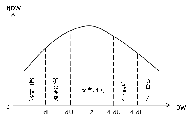
Durbin-Watson d test: $$d=\frac{\sum\limits_{t=2}^{n}(e_{t}-e_{t-1})^{2}}{\sum\limits_{t=1}^{n}e_{t}^{2}}$$
- Requests:
  - Regression model includes intercept.
  - $X$ are nonstochastic.
  - Error term $u_{i}$ follows: $u_{t}=\rho u_{t-1}+v_{t}\quad -1\leq\rho\leq1$
  - $\rho$ is called coefficient of autocorrelation. This equation is called Markov first-order autoregressive scheme, deneted as $AR(1)$.
  - Variables doesn’t include the lag term of $Y$ (not autoregressive models).
- Large sample – $d\approx2(1-\hat{\rho}),\hat{\rho}=\frac{\sum\limits_{t=2}^{n}e_{t}e_{t-1}}{\sum\limits_{t=1}^{n}e_{t}^{2}}$. So $0\leq d\leq4$.
- $\hat{\rho}\rightarrow -1\text{ (negative correlation)},d\rightarrow 4$.
- $\hat{\rho}\rightarrow 0\text{ (no correlation)},d\rightarrow2$.
- $\hat{\rho}\rightarrow 1\text{ (positive correlation)},d\rightarrow 0$.
- There are two critical value $d_{L},d_{U}$.

0.6.3 Solutions

GLS
- Suppose error term follows $AR(1)$: $u_{t}=\rho u_{t-1}+v_{t}$.
- OLS regress $Y_{t}^{*}=B_{1}^{*}+B_{2}^{*}X_{t}^{*}+v_{t}$.
- $Y_{t}^{*}=Y_{t}-\rho Y_{t-1}$, the others are similar.
- This method is called Generalized Least Squares, GLS, this equation is called Generalized Difference Equation.
- The first instance is lost in this difference equation, we can transform it using this fomular (Prais-Winsten transformation):
- $Y_{1}^{*}=\sqrt{1-\rho^{2}}(Y_{1}),X_{1}^{*}=\sqrt{1-\rho^{2}}(X_{1})$.
- The estimation of $\rho$.
  - $\rho=1$: first-order difference method, suppose error term are positively correlated.
  - Estimate $\rho$ from Durbin-Watson d statistic. $d\approx2(1-\hat{\rho})\Rightarrow\hat{\rho}\approx1-\frac{d}{2}$.
  - Estimate $\rho$ from OLS residuals $e_{t}$: $e_{t}=\hat{\rho}e_{t-1}+v_{t}$.
Large sample method: Newey-West method
- Also HAC std. It doesn’t advise the values of OLS estimators, but just advise their stds.

Haohan Zhao